QZS L6 Tool output format change

category: gnss

Table of contents

Introduction

I have released a tool QZS L6 Tool that displays messages broadcast by positioning satellites.

This name comes from the L6 frequency band of the quasi-zenith satellite (QZS). QZS broadcasts in the L6 frequency band CLAS (pronounced as same as Cirrus, centimeter-level augmentation service). I made it because I wanted to know how accurate positioning works. After the first relase, QZS L6 Tool became able to read messages from Galileo’s HAS (high accuracy service) and BeiDou’s PPP-B2b (precise point positioning - B2b-signal).

However, because the display format was “item = value”, it was difficult to reuse and compare messages between systems. Therefore, I changed the output format with the aim of making the QZS L6 Tool output both machine-readable and human-readable.

In the process of reviewing the QZS L6 Tool code, I reread the CLAS specifications and fixed some bugs in the codes. While I realized that there were parts of the specification description that I had misinterpreted, I took note of the parts that I still don’t understand (if anyone knows, please let me know.).

Download

QZS L6 Tool can also be downloaded in ZIP format. However, downloading using git is recommended for upgrades. To download using git, run:

git clone https://github.com/yoronneko/qzsl6tool

If it was already downloaded using git, running git pull in that directory will upgrade it. Even if you make your own improvements, git will update you as much as possible to track your changes, and it’s convenient because it can clearly display changes to specific code.

Change in display format

Using QZS CLAS as an example, compare this display format change in the screenshot below (left: before change, right: after change). For example, in the ST2 (subtype 2, satellite orbit correction) display, the number of characters per line has been reduced, making it easier to read.

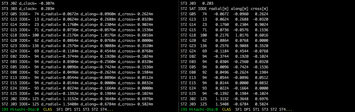
QZS L6 Tool display style modification

The new format displays a heading (for example, ST2 SAT IODE radial[m] along[m] cross[m]) at the beginning of each data column. For satellite time correction, clock and c0 were used together, but since they both refer to the same thing, they were unified to c0 (for satellite time correction, c1 and c2 are also sometimes used). In addition, CLAS now displays not only the network ID but also the area name, and latitude and longitude coordinates instead of a grid.

This change is useful for organizing material. As an example, we will process data from the high-precision augmentation information PPP-B2b broadcast by the Chinese positioning satellite BeiDou. sample/20230819-081730hasbds.sept in QZS L6 Tool has data that I obtained with a Septentrio mosaic-go X5 receiver. The result of processing this with test/do_test.sh is test/expected/20230819-081730hasbds.b2b.txt. Some of this content is as follows:

C60 MT4  CLOCK 08:17:34 IODSSR=1 IODP=2
SAT IODCorr   c0[m]
C19       4   0.483
C20       4  -0.035
C23       6  -0.050
C60 MT4  CLOCK 08:17:34 IODSSR=1 IODP=2
SAT IODCorr   c0[m]
C24       6  -0.178
C26       4   0.000
C35       2   1.682
C37       3  -0.920
C39       2   0.339
C42       1   0.578
C45       0   0.443

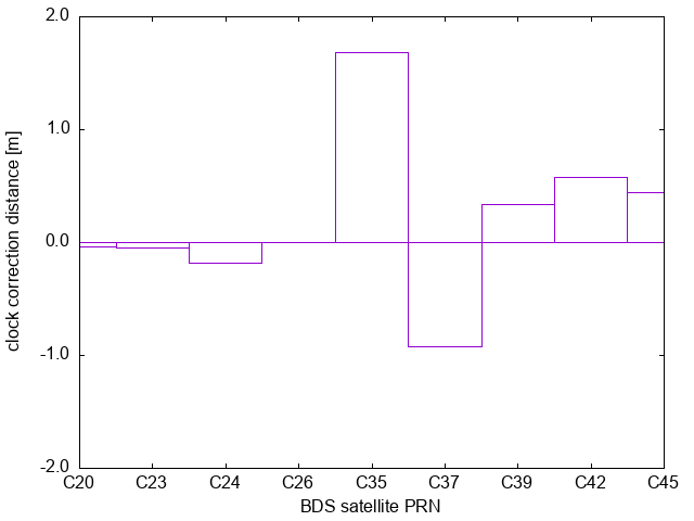
This is clock correction information (MT4) broadcast by BeiDou’s geostationary satellite C60, and is for C19 satellite, C20 satellite, and others. The first column shows the satellite number, the second column displays the data management number, and the third column is for the satellite clock correction in meters (clock correction usually is expressed in meters, by multiplied by the speed of light to the clock difference).

We copy this part and display it using the graph display software gnuplot. Create a script file (for example, ppp-b2b.gp) with the following content, paste the previous data between $data << EOD and EOD (the string EOD can be another string as you like), and make a slight format change to the pasted part.

ppp-b2b.gp

# -*- coding: utf-8 -*-
# gnuplot script
# clock correction distance, source:
# directory of test/expect/20230819-081730hasbds.b2b.txt of
# QZS L6 Tool, https://github.com/yoronneko/qzsl6tool.

$data << EOD
# SAT IODCorr   c0[m]
C19       4   0.483
C20       4  -0.035
C23       6  -0.050
C24       6  -0.178
C26       4   0.000
C35       2   1.682
C37       3  -0.920
C39       2   0.339
C42       1   0.578
C45       0   0.443
EOD

set termoption enhanced
set termoption font "Times New Roman, 18"
set termoption linewidth 3
set border lw 0.5
set yrange[-2:2]; set ytics 1
set format y "%3.1f"
set xlabel "BDS satellite PRN"
set ylabel "clock correction distance [m]"
set key off
plot $data u (column(0)):3:xtic(1) ti col with boxes

# EOF

This format change involves commenting out the beginning of the heading line and deleting heading lines between data that spans multiple lines. In gnuplot, lines starting with # in script files are considered commented out and ignored.

Run gnuplot, load this script file, and boxplot. The graph is displayed with load "ppp-b2b.gp, and the graph is converted to a PNG file with set output "ppp-b2b.png" set term png rep It will be saved in ppp-b2b.png and gnuplot will be terminated with quit.

QZS L6 Tool display style modification

$ gnuplot -d

	G N U P L O T
	Version 6.0 patchlevel 0    last modified 2023-12-09

	Copyright (C) 1986-1993, 1998, 2004, 2007-2023
	Thomas Williams, Colin Kelley and many others

	gnuplot home:     http://www.gnuplot.info
	faq, bugs, etc:   type "help FAQ"
	immediate help:   type "help"  (plot window: hit 'h')

	Terminal type is now qt
gnuplot> load "ppp-b2b.gp"
gnuplot> set output "ppp-b2b.png"
gnuplot> set term png

Terminal type is now 'png'
Options are 'truecolor nocrop enhanced butt size 640,480 font "arial,12.0" '
gnuplot> rep
gnuplot> quit

Of course, you can also save the data to a file and plot it, or specify PDF as the plot file format.

After creating a graph, changing the graph display format, axis names, aspect ratio, replacing data content, and creating many graphs with large amounts of data are common daily occurrences for researchers and students. Don’t get angry if your professor or boss tells you as:

Align the display ranges of the vertical and horizontal axes of all graphs.
Make the numerical intervals 1, 2, or 5.
Remake all graphs!

To recreate the graph with gnuplot, you just need to modify the script file and load that file. It would be a good idea to have the generation AI create a batch file that processes many data files at once. gnuplot is more convenient than Excel for creating graphs. If you choose to create a report in LaTeX, it is possible to completely automate graph replacement (which is what I do!).

gnuplot can be easily installed using the following method：

If you use the Mac’s package manager homebrew, use brew install gnuplot.
If you use the Windows standard package manager winget, use winget install gnuplot.gnuplot.
If you use the Linux distributions’ standard package manager apt, use apt install gnuplot.

What I didn’t understand about the CLAS specifications

CLAS Specification (IS-QZSS-L6-005), Explanation materials (in Japanese), sample program (CLASLIB) are provided on the QZS official page.

In the process of reviewing the QZS L6 Tool code, I remembered something that I didn’t understand in the CLAS specification.

How to find the beginning of the frame. In the L6D signal in which CLAS is transmitted, one data part (DP, 2000 bits) is transmitted every second. The receiver collects 5 parts of the DP to obtain a subframe (SF), and further collects 6 subframes of SF to obtain a frame forming one period, and interprets the contents. The header of each DP has a subframe indicator (1-bit length) that indicates the beginning of SF, and the beginning of SF can be identified. However, there doesn’t seem to be an official way to identify the beginning of a frame. In QZS L6 Tool, if there is mask information (subtype 1) at the beginning of an SF, that SF is regarded as the beginning of the frame. This is because without the mask information, the information cannot be decoded. If this way is correct, I am grateful if the method is explicitly written in Section 4.1.2.2.1 (page 24) of the specification.
How to handle “not available” for decoding data. For example, when the GNSS Hourly Epoch value of subtype 2 is 3600 or more, it indicates unavailability. Even in that case, it is natural to read the following data such as SSR Update Interval. However, for example, when data indicating unavailability is stored in subtype 8 STEC Polynomial Coefficient C00, the following C01 and C10 are meaningless. At this time, I am not sure that data indicating unavailability be stored in C01 and C10 as well. Or, in this case, because C01 and C10 are meaningless, and they don’t be transmitted, then the current QZS L6 Tool will not be able to read SF data after that. I would be grateful if it was written in the Note section that following data that becomes meaningless due to previous data unavailability is always stored with data indicating unavailable.
CLAS calculates the pre-hardcoded reference coordinate values in Section 4.1.4 (page 71) of the specification from the compact network ID and grid ID. First, the receiver uses this set of reference coordinate values to find the network ID and grid ID that are closest to the rough coordinates of the location we want to observe. At this time, I am not sure how determine the distance threshold between the observation point coordinate value and the reference coordinate value. When we use CLAS at sea, I would be grateful if a reference value for this threshold is provided in section 4.1.4 of the specifications in order to avoid using distant reference points.
How to read subtype 12 STEC data. Two bits are assigned for subtype 12 STEC Correction Availability (not STEC Corretion Type) (Specification Section 4.1.2.2.13, Table 4.1.2-35, page 52). However, (2) on page 56 of the specification only describes the operation of the first bit. If this second bit is reserved and is always set to zero, I would be grateful if it is written as such in (2) on page 56.
How to convert STEC Quality Indicator to STEC Quality. As an explanation for subtype 8, section 4.1.2.29 (page 43) of the specification states, “The definition is the same as that for SSR URA whereas the dimension is TECU instead of m”. Therefore, we may use the same formula for obtaining both URA and STEC Quality from the 6-bit indication value. However, the URA value written in Table 5.4.2-1 (page 81) in section 5.4.2 and the TECU values written in Table 5.4.3-1 (page 84) in section 5.4.3 are different. Section 5.4.2 contains not only values but also calculation formula, but section 5.4.3 does not contain calculation formula. It does not seem that the STEC values are come from the URA by dividing a certain value. I would be grateful if Section 5.4.3 of the specification describes the formula for calculating STEC Quality from the STEC Quality Indicator.

These questions may be answered by reading the CLASLIB source code. CLASLIB is a big piece of software, and I actually gave up on reading it halfway through. I’m very grateful that the source code is open to the public, so I’d like to read it little by little.

If you use CLAS, you can experience its greatness. I am very grateful that this is available for free in Japan.

Conclusion

QZS L6 Tool output is in tabular format, aiming to be both machine-readable and human-readable. I have also summarized how to use it. Also, I have summarized my questions regarding the CLAS specification. git and gnuplot are very useful.

Positioning satellites are all around us. The high-precision positioning augmentation services of CLAS, MADOCA-PPP, SLAS, Galileo HAS, BeiDou PPP-B2b, and SBAS are all excellent. I am grateful that these advanced technologies are available to anyone for free.