Quantitative evaluation of sky visibility using a spherical camera

Introduction

When conducting outdoor experiments of satellite positioning or wireless communication, it is easier to explain the environment if the sky obstruction caused by such as the terrain or buildings can be expressed numerically. I calculated the sky-view factor (SVF, the percentage of the sky that can be seen) from image files taken with an omnidirectional camera with Python code.

Spherical camera

A spherical camera can capture an entire scene in one shot. It captures multiple images simultaneously using an image sensor equipped with wide-angle lenses, stitches these images together, and captures the entire scene in one photo.

The stitched image is output as a standard JPEG image file, so it can be viewed on a regular computer or smartphone. However, since this image was taken with a wide-angle lens, it appears curved as is. This image file can be displayed in VR using the camera’s attached app, but since it is a representation format equivalent to the Mercator projection familiar from maps, many people are trying to convert it into various image formats.

Here, I use a Ricoh Theta V equipped with two wide-angle lenses. This camera is very convenient because it can perform zenith correction of images using an attitude sensor, and can also use a remote shutter with a smartphone app. For example, the 3D panoramic photos of the Hiroshima City University RTK reference station are rendered using JavaScript.

Calculation of sky-view factor

Here, we consider bright areas of the image to be sky, and calculate the percentage of sky in the image. This brightness threshold is calculated using Otsu’s binarization method.

The sky visibility factor (SVF) is calculated by the following steps: (1) cutting the upper hemisphere from the horizon to the zenith, assuming vertical correction, (2) converting from equidistant cylindrical projection to equidistant and equal-area projection, (3) grayscaling, (4) determining the brightness threshold using Otsu’s binarization method, (5) performing binarization, and (6) calculating the percentage of pixels exceeding the threshold. For this image processing, OpenCV and the Python modules numpy, pillow, and scikit-image are used.

pip install pillow scikit-image

The Python code skyview.py created here is as follows. The -f option outputs a fisheye image, the -b option outputs a binarized image, and the -t option adjusts the binarization threshold.

#!/usr/bin/env python
# -*- coding: utf-8 -*-
# This file is for sky view factor calculation
# pip install pillow scikit-image

from PIL import Image
import numpy as np
import matplotlib.pyplot as plt
import sys
import argparse
from scipy.ndimage import map_coordinates
from skimage.filters import threshold_otsu
from skimage.color import rgb2gray

def remap_equidistant_to_fisheye_array(img, fov_deg=180):
    # Calculate the new dimensions for the square fisheye image
    # Assuming the field of view is a full hemisphere
    fov = np.radians(fov_deg)
    h, w = img.shape[:2]
    w_new = int(w * fov / np.pi)
    h_new = w_new

    # Define the new image with the same channel count as the original
    fisheye_img = np.zeros((h_new, w_new, img.shape[2]), dtype=img.dtype)

    # Coordinates of the new image
    xx_new, yy_new = np.meshgrid(np.arange(w_new), np.arange(h_new))

    # Re-center the coordinates at the center of the fisheye image
    xx_new = xx_new - w_new / 2.0
    yy_new = yy_new - w_new / 2.0

    # Calculate the r, theta coordinates
    r = np.sqrt(xx_new**2 + yy_new**2)
    theta = np.arctan2(-yy_new, xx_new) + np.pi

    # Calculate the corresponding coordinates in the source image
    xx = (w * theta / (2 * np.pi)).astype(np.float32)
    yy = (h * r / r.max()).astype(np.float32)

    # Map the polar coordinates back to the cylindrical coordinates
    map_x = xx.clip(0, w-1)
    map_y = yy.clip(0, h-1)

    # Use scipy's map_coordinates for efficient remapping
    for i in range(img.shape[2]):
        fisheye_img[:, :, i] = map_coordinates(img[:, :, i], [map_y.flatten(), map_x.flatten()], order=1).reshape((h_new, w_new))

    return Image.fromarray(fisheye_img)


if __name__ == '__main__':
    parser = argparse.ArgumentParser(description='Calculate the sky view factor of a fisheye image')
    parser.add_argument('images', type=str, nargs='+', help='Path to the original image')
    parser.add_argument('-f', '--fisheye', action='store_true' , help='switch to save fisheye image')
    parser.add_argument('-b', '--binary', action='store_true', help='switch to save binary image')
    parser.add_argument('-t', '--threshold', type=float, default=0.0, help='threshold offset')
    args = parser.parse_args()
    for image in args.images:  # For each image in the command line arguments
        # Path to the original image
        img_original = np.array(Image.open(image))

        # Cut the original image to only keep the sky
        img_sky = img_original[:img_original.shape[0] // 2, :]

        # Convert the sky part to fisheye
        fisheye_sky_image = remap_equidistant_to_fisheye_array(img_sky)

        # Save the fisheye sky image
        if args.fisheye:
            path_image_fisheye = image.split('.')[0] + '_fish.jpg'
            fisheye_sky_image.save(path_image_fisheye)

        # Convert the image to grayscale for thresholding
        gray_fisheye_sky_image = rgb2gray(fisheye_sky_image)

        # Find the Otsu threshold value
        threshold_value = threshold_otsu(gray_fisheye_sky_image)
        threshold_value += args.threshold

        # Apply the threshold to binarize the image
        binary_fisheye_sky_image = gray_fisheye_sky_image > threshold_value

        # Calculate the proportion of sky and clouds
        # Assuming that sky is white after thresholding
        sky_ratio = np.sum(binary_fisheye_sky_image) / binary_fisheye_sky_image.size

        if args.binary:
            path_image_sky = image.split('.')[0] + '_bin.jpg'
            # Convert the binary image back to uint8 for saving
            binary_fisheye_sky_image = (binary_fisheye_sky_image * 255).astype(np.uint8)
            binary_fisheye_sky_image = Image.fromarray(binary_fisheye_sky_image)

            # Save the binary image
            binary_fisheye_sky_image.save(path_image_sky)

        print(f'{image} sky ratio: {sky_ratio * 100:.1f}%')

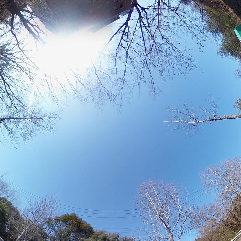
We will calculate SVF using the following photo taken with a spherical camera as an example.

240318-144315.jpg

To organize a lot of images, I set the internal time on my camera and use jhead to rename JPEG files to include the date and time based on the EXIF ​​(Exchangeable image file format) information (jhead -nf%y%m%d-%H%M%S -autorot *.jpg). jhead can be easily installed with brew install jhead on Mac, or apt install jhead -y on Debian Linux.

We will process this image file 240318-144315.jpg, which was taken on 2024-03-18 14:43:15 JST.

$ ./skyview.py -f -b 240318-144315.jpg
240318-144315.jpg sky ratio: 52.4%

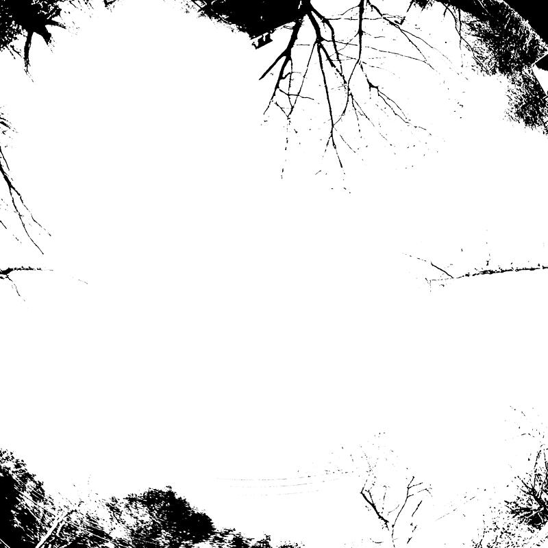
The SVF was evaluated as 52.4%. The output fisheye image 240318-144315_fish.jpg and binarized image 240318-144315_bin.jpg are as follows.

240318-144315_fish.jpg 240318-144315_bin.jpg

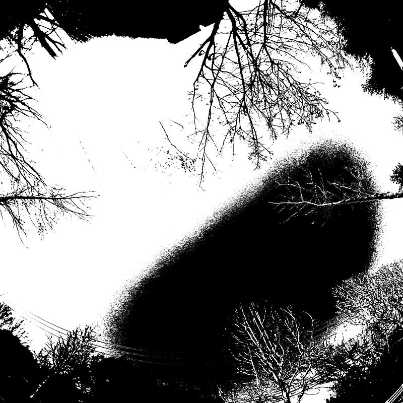
In the binarized image, the obvious sky areas are treated as occluded. Therefore, I repeatedly adjusted the threshold and displayed the binarized image so that the sky areas could be recognized as sky. Finally, I selected -0.30 as the binarization threshold for this image and evaluated its SVF as 92.2%.

$ ./skyview.py -b -t -0.30 240318-144315.jpg
240318-144315.jpg sky ratio: 92.2%

240318-144315_bin.jpg

With this threshold, some parts of the building were considered to be empty. I think this is the limit of what can be achieved by adjusting the threshold alone.

Obvservation of sky-view factor

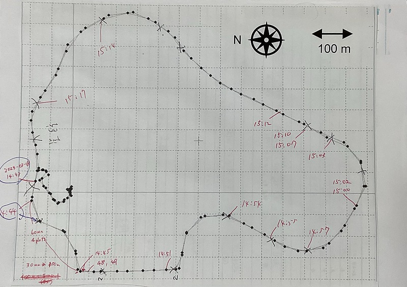
I took my spherical camera and smartphone outside to observe the sky visibility of the roads around my workplace. I drove around the roads around my university while using the GPS receiver in my car to determine my position, and plotted the course I took using rtkplot.exe from RTKLIB and printed it out.

A spherical camera is set up along the driving course, and photos are taken remotely using a smartphone app, with the time of the photos being recorded on the course.

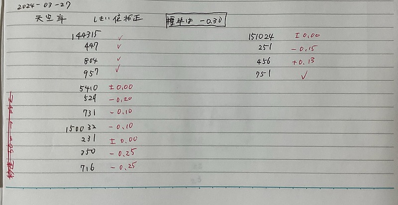
After that, I downloaded the image files from the spherical camera to my PC and renamed them to include the date and time using the method using jhead mentioned above. I then created the following shell script, ran the above skyview.py on all the image files, compared the fisheye images and binary images, and adjusted the threshold. It’s a pretty analog method.

./skyview.py -b -f -t -0.30 240318-144315.jpg
./skyview.py -b -f -t -0.30 240318-144447.jpg
./skyview.py -b -f -t -0.30 240318-144804.jpg
./skyview.py -b -f -t -0.30 240318-144957.jpg
./skyview.py -b -f -t -0.00 240318-145410.jpg
./skyview.py -b -f -t -0.20 240318-145529.jpg
./skyview.py -b -f -t -0.10 240318-145731.jpg
./skyview.py -b -f -t -0.10 240318-150032.jpg
./skyview.py -b -f -t  0.00 240318-150231.jpg
./skyview.py -b -f -t -0.25 240318-150350.jpg
./skyview.py -b -f -t -0.25 240318-150716.jpg
./skyview.py -b -f -t  0.00 240318-151024.jpg
./skyview.py -b -f -t -0.15 240318-151251.jpg
./skyview.py -b -f -t  0.13 240318-151456.jpg
./skyview.py -b -f -t -0.30 240318-151751.jpg

The SVF on this driving course was calculated by this way.

240318-144315.jpg sky ratio: 92.2%
240318-144447.jpg sky ratio: 88.3%
240318-144804.jpg sky ratio: 91.4%
240318-144957.jpg sky ratio: 94.5%
240318-145410.jpg sky ratio: 64.9%
240318-145529.jpg sky ratio: 76.0%
240318-145731.jpg sky ratio: 74.7%
240318-150032.jpg sky ratio: 72.8%
240318-150231.jpg sky ratio: 63.9%
240318-150350.jpg sky ratio: 88.4%
240318-150716.jpg sky ratio: 85.8%
240318-151024.jpg sky ratio: 53.2%
240318-151251.jpg sky ratio: 78.7%
240318-151456.jpg sky ratio: 69.3%
240318-151751.jpg sky ratio: 85.0%

Then, based on the time information in the file name, the SVF values ​​were written to the driving course.

I was hoping that the smartphone coordinates would be automatically recorded in the EXIF ​​information of these JPG image files, but there was no such record.

$ jhead 240318-144315.jpg
File name    : 240318-144315.jpg
File size    : 4950603 bytes
File date    : 2024:03:18 21:07:33
Camera make  : RICOH
Camera model : RICOH THETA V
Date/Time    : 2024:03:18 14:43:15
Resolution   : 5376 x 2688
Flash used   : No
Focal length :  1.3mm
Exposure time: 0.0008 s  (1/1250)
Aperture     : f/2.0
ISO equiv.   : 64
Whitebalance : Auto
Metering Mode: pattern
Exposure     : program (auto)
JPEG Quality : 95
======= IPTC data: =======
City          :
Record vers.  : 2
Time Created  : 144315+0900
Caption       :
DateCreated   : 20240318

In the future, I would like to install a spherical camera and a GPS receiver on the roof of a car, and automatically calculate the driving course and SVF from the video. I would also like to record images so that the front of the spherical video always faces due north, using a GPS receiver that can obtain heading information such as a Unicore UM982 receiver and image processing.

Conclusion

I calculated the sky-view factor (SVF) from the image of the spherical camera. I used Otsu’s binarization method to calculate the sky ratio, but it became necessary to adjust the threshold while looking at the image. I identified the shooting location based on the shooting time information and associated the shooting location with the SVF. Since there are many manual parts, I would like to consider automating this process in the future.