Galileo HAS Reference User Algorithm in Matlab
Introduction
By receiving the signals broadcast by Global Navigation Satellite Systems (GNSS), such as the US GPS, the European Union’s (EU) Galileo, and Japan’s Quasi-Zenith Satellite System “Michibiki,” we can estimate our own position. Methods that improve positioning accuracy by correcting the satellite positions, time, and pseudoranges from the satellites to the receiver obtained from these signals are called augmentation.
Galileo provides an augmentation service called HAS (High Accuracy Service). Its augmentation information is transmitted on the E6-B signal of Galileo satellites and is also distributed over the Internet. HAS is free for anyone to use, and its signal specification is publicly available.
The European GNSS Service Centre (GSC) has released the performance evaluation software “HAS Reference User Algorithm” together with sample data for HAS, so I tried it out.
Obtaining the software and sample data
The software requires MATLAB and its Statistics and Machine Learning Toolbox. On Windows, installing the Parallel Computing Toolbox also allows the computation to run in parallel, reducing processing time.
I learned of the release of the software and data through the GSC mailing list and applied for it on June 20, 2026.
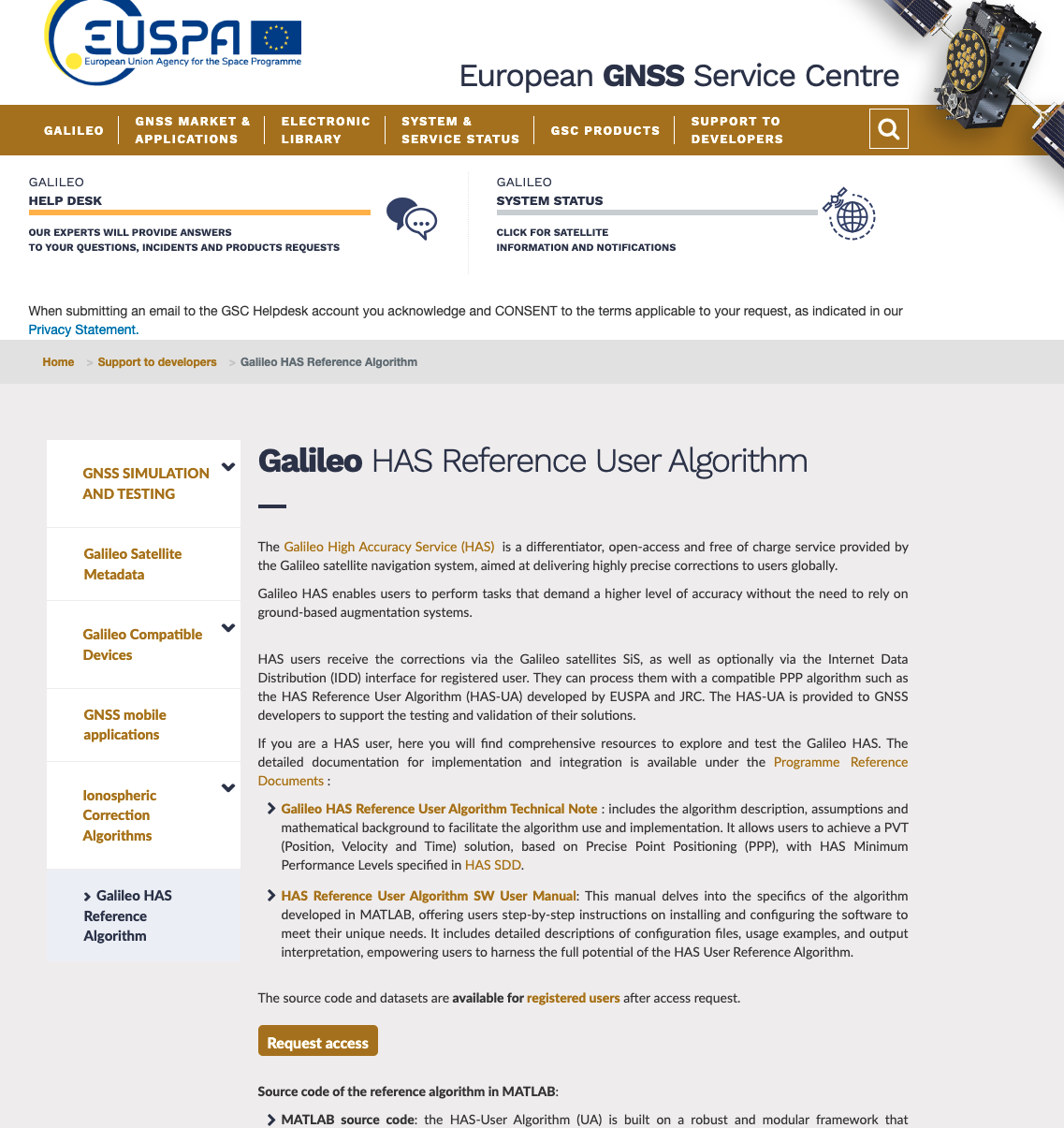
To apply, you first need to register a GSC account. After registering, log in and click the “Request access” button shown below.
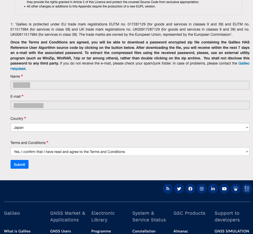
Read the license agreement on the next page. At the bottom, enter your name and email address, select your country, accept the license, and press the “Submit” button.
The following page shows a download link for a ZIP file. The file is about 3.5 GB and password-protected. In my environment, the download took half a day. The password for the ZIP file arrived by email about a week later.
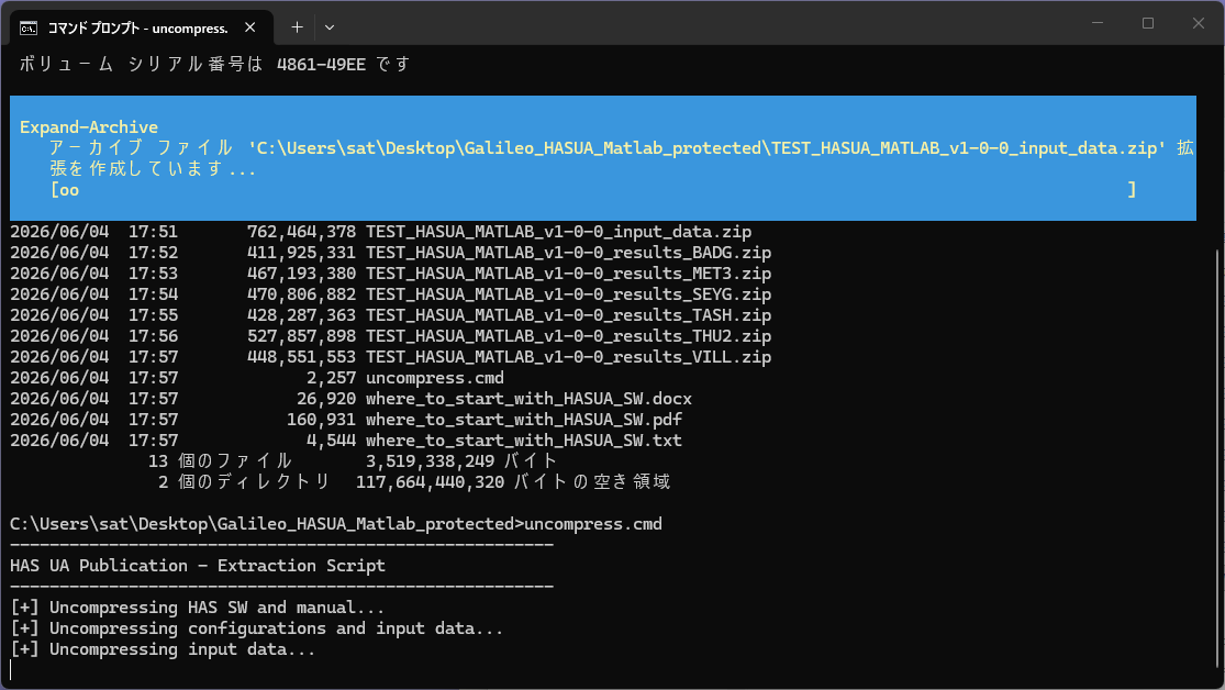
After obtaining the password and extracting the ZIP file, I found several more ZIP files, a Windows extraction script uncompress.cmd, and a file describing how to use the software.
All of these ZIP files must be extracted while preserving the directory structure. I first tried Keka, an archive utility on the Mac, but found it difficult to preserve the directory structure. In the end, I ran uncompress.cmd from the Command Prompt on a Windows PC. The extracted files total about 7 GB. Since the source code is written as MATLAB M-files (plain text), it basically works the same way on both Windows and Mac (see below for notes on the Mac).
Directory structure
The top directory contains the following two M-files and four subdirectories: conf, data, doc, and src.
- Example_Run_HASUA_PPPSD_stat_year_doy_all.m (computation program)
- Example_Plot_HASUA_PPPSD_stat_year_doy_any.m (result plotting program)
The sample data is in the data directory. It contains directories of RINEX observation data for each station (station names BADG, MET3, SEYG, TASH, THU2, and VILL), as well as a common directory containing RINEX navigation data, augmentation data, and antenna information (ANTEX).
Each directory is divided by year (2023 only here) and by DOY (day of year, counting January 1 as day 1; 356 to 365 here). The computation results are stored in directories beginning with results_ inside these directories.
Positioning for each observation data set is computed for a total of six cases: three signal combinations, Galileo E1-E5a, GPS L1-L2, E1-E5b, L1-L2, and E1-E6, L1-L2, combined with two augmentation sources, Internet distribution IDD (Internet Data Distribution) and distribution via the E6-B signal SIS (Signal-in-Space).
Three types of output files, with the computation date and time in their file names, are produced: a result file in MAT format, a text result file with the extension .sol, and a log file with the extension .log. The result directories also contained precomputed result files (for example, BADG00RUS_R_20233560000_01D_30S_MO_PPPSD_160120_SSRC_SIS_2026_04_28_12_59_12.mat).
data
├── BADG
│   └── 2023
│       ├── 356
│       │   ├── results_E1_E5a_L1_L2_IDD
│       │   ├── results_E1_E5a_L1_L2_SIS
│       │   ├── results_E1_E5b_L1_L2_IDD
│       │   ├── results_E1_E5b_L1_L2_SIS
│       │   ├── results_E1_E6_L1_L2_IDD
│       │   └── results_E1_E6_L1_L2_SIS
│       ├── 357
...
├── common
│   └── 2023
│       ├── 356
│       ├── 357
│       ├── 358
│       ├── 359
│       ├── 360
│       ├── 361
│       ├── 362
│       ├── 363
│       ├── 364
│       └── 365
├── MET3
...
The src directory contains the source code. In MATLAB, each function is written in its own M-file. Counting the M-files in the src directory with the following command gives 383, which shows that this is a large program.
find src -name '*.m' | wc -l
383
Sample data
The common directory contains 10 days of RINEX navigation data. The beginning of the RINEX file for DOY 356 (2023-12-22) is shown below.
     3.05           NAVIGATION DATA     MIXED               RINEX VERSION / TYPE
BCEmerge            congo               20231222 004605 GMT PGM / RUN BY / DATE
gfzrnx-2.1.9        FILE MERGE          20241112 113001 UTC COMMENT
BDSA   4.1910e-08  3.7253e-08 -1.0133e-06  1.6093e-06       IONOSPHERIC CORR
BDSB   1.1469e+05  1.8022e+05 -1.8350e+06  1.9661e+06       IONOSPHERIC CORR
GAL    1.4300e+02 -8.9844e-01  5.5237e-03           0       IONOSPHERIC CORR
GPSA   2.6077e-08  7.4506e-09 -1.1921e-07  1.1921e-07       IONOSPHERIC CORR
GPSB   1.4950e+05 -2.1299e+05  0.0000e+00  3.2768e+05       IONOSPHERIC CORR
IRNA   8.1025e-08  2.9802e-07 -2.8610e-06 -7.5102e-06       IONOSPHERIC CORR
IRNB   1.2493e+05  7.3728e+05 -2.0972e+06 -8.3231e+06       IONOSPHERIC CORR
QZSA   6.6124e-08 -7.0035e-07  1.9670e-06  0.0000e+00       IONOSPHERIC CORR
QZSB   7.9872e+04  1.1960e+06 -8.3886e+06 -8.3886e+06       IONOSPHERIC CORR
GAGP  9.6042640507e-10 8.881784197e-16 432000 2293          TIME SYSTEM CORR
GAUT -1.8626451492e-09 8.881784197e-16 345600 2293          TIME SYSTEM CORR
GLGP -3.9115548134e-08 0.000000000e+00 345600 2293          TIME SYSTEM CORR
GLUT  9.3132257462e-10 0.000000000e+00 345600 2293          TIME SYSTEM CORR
GPUT  0.0000000000e+00 4.440892099e-15  61440 2294          TIME SYSTEM CORR
IRGL  5.5530108511e-08-4.440892099e-14 430800 2293          TIME SYSTEM CORR
IRGP  4.5984052122e-09-1.332267630e-15 430800 2293          TIME SYSTEM CORR
QZUT  4.6566128731e-09 0.000000000e+00   8192 2294          TIME SYSTEM CORR
    18    18  1929     7                                    LEAP SECONDS
This navigation data also includes data for China’s BeiDou, Japan’s Michibiki, and India’s NavIC.
The station directories, such as BADG and MET3, contain 10 days of RINEX observation data. As an example, the beginning of the RINEX file for station BADG on DOY 356 is shown below.
     3.04           OBSERVATION DATA    M                   RINEX VERSION / TYPE
JPS2RIN v.2.0.178   JAVAD GNSS          20231223 000638 UTC PGM / RUN BY / DATE
AUTOMATIC           IAA                                     OBSERVER / AGENCY
BADG                                                        MARKER NAME
12338M002                                                   MARKER NUMBER
02682               JAVAD TRE_3 DELTA   3.7.10 Oct,22,2020  REC # / TYPE / VERS
  -838282.9631  3865774.0774  4987620.6604                  APPROX POSITION XYZ
00328               JAVRINGANT_DM   JVDM                    ANT # / TYPE
        0.0280        0.0000        0.0000                  ANTENNA: DELTA H/E/N
G   20 C1C L1C D1C S1C C1W L1W D1W S1W C2X L2X D2X S2X C2W  SYS / # / OBS TYPES
       L2W D2W S2W C5X L5X D5X S5X                          SYS / # / OBS TYPES
R   20 C1C L1C D1C S1C C1P L1P D1P S1P C2C L2C D2C S2C C2P  SYS / # / OBS TYPES
       L2P D2P S2P C3X L3X D3X S3X                          SYS / # / OBS TYPES
E   20 C1X L1X D1X S1X C8X L8X D8X S8X C6X L6X D6X S6X C7X  SYS / # / OBS TYPES
       L7X D7X S7X C5X L5X D5X S5X                          SYS / # / OBS TYPES
 26 R01  1 R02 -4 R03  5 R04  6 R05  1 R06 -4 R07  5 R08  6 GLONASS SLOT / FRQ #
    R09 -2 R10 -7 R11  0 R12 -1 R13 -2 R14 -7 R15  0 R16 -1 GLONASS SLOT / FRQ #
    R17  4 R18 -3 R19  3 R20  2 R21  4 R22 -3 R23  3 R24  2 GLONASS SLOT / FRQ #
    R25 -5 R26 -6                                           GLONASS SLOT / FRQ #
    30.000                                                  INTERVAL
  2023    12    22     0     0    0.0000000     GPS         TIME OF FIRST OBS
  2023    12    22    23    59   30.0000000     GPS         TIME OF LAST OBS
    18                                                      LEAP SECONDS
This shows that observations were made every 30 seconds over 24 hours. HAS augments Galileo and GPS, but the observation data also included Russia’s GLONASS.
The coordinates of each station, which serve as the ground truth for high-accuracy positioning, are written in ECEF (Earth-Centered, Earth-Fixed) form in the result plotting program Example_Plot_HASUA_PPPSD_stat_year_doy_any.m. I converted them to latitude, longitude, and ellipsoidal height with ecef2llh.py from QZS L6 Tool and summarized them below.
$ ecef2llh.py -.838282176007901E+06 0.386577732440940E+07 0.498762455124815E+07
51.7697041 102.2349908 811.421
| station name | latitude [deg] | longitude [deg] | ellipsoidal height [m] | Google Maps link |
|---|---|---|---|---|
| BADG | 51.7697041 | 102.2349908 | 811.421 | Badary RTF-32, Russia |
| MET3 | 60.2174569 | 24.3945036 | 79.232 | Metsähovi Geodetic Research Station, Finland |
| SEYG | -4.6787305 | 55.5306332 | -37.619 | Seychelles International Airport? |
| TASH | 41.3280498 | 69.2955723 | 439.713 | Teleskop, Uzbekistan |
| THU2 | 76.5370484 | -68.8250532 | 36.238 | Dundas?, Greenland |
| VILL | 40.4435961 | -3.9519751 | 647.341 | European Space Agency, Spain |
HAS computation and result plots
The computation uses Example_Run_HASUA_PPPSD_stat_year_doy_all.m in the top directory. The observation data covers 6 stations over 10 days, each with 6 combinations of signals and distribution paths, for a total of 360 computations. Running this program performs positioning for one day at 30-second intervals (2880 epochs) for each of them.
I tried it on several machines, including a Mac desktop with an Apple Silicon M1 and 16 GB of memory and a Windows desktop with a Core i3-8100 and 32 GB of memory. On each of them, processing one observation data set took about 360 seconds. In my Windows environment, the Parallel Computing Toolbox ran only two workers in parallel. On the Mac, having this toolbox installed causes an error indicating that the memory function is unavailable. On a Mac with the Parallel Computing Toolbox installed, I had to add has_parallel=false to the source code so that the toolbox would not be used.
In fact, I could not complete all the computations on my PCs. I left them running when I went home, and when I came back to work the next day, the PCs had rebooted or their displays were corrupted, and the computation had stopped.
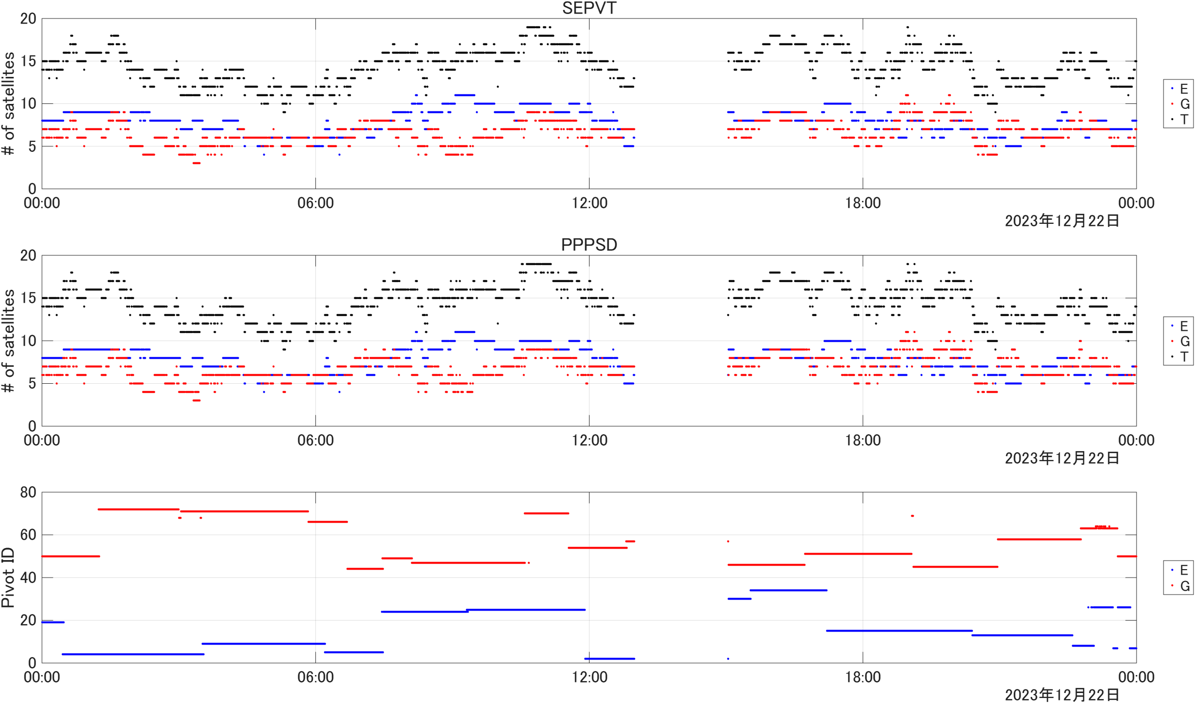
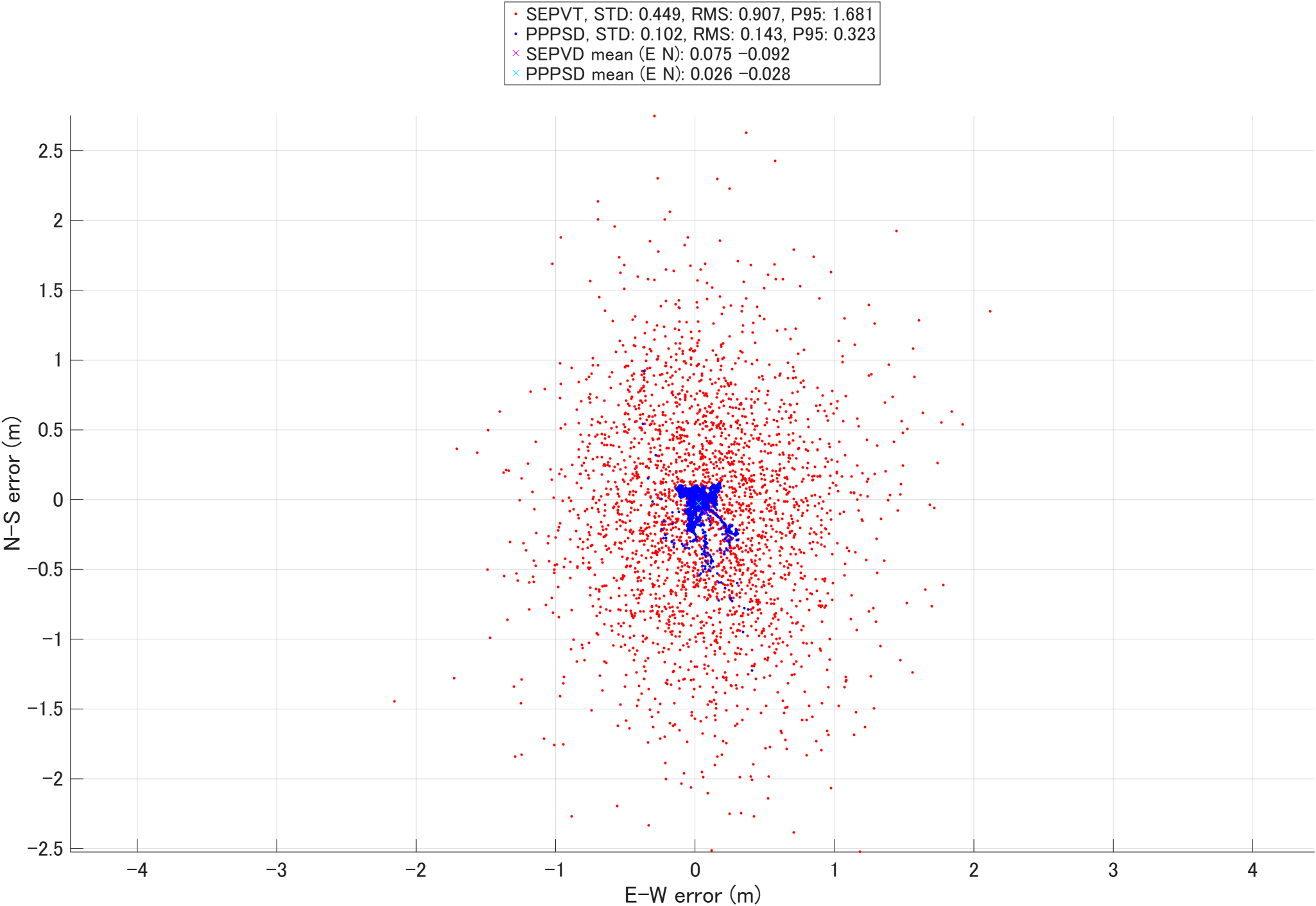
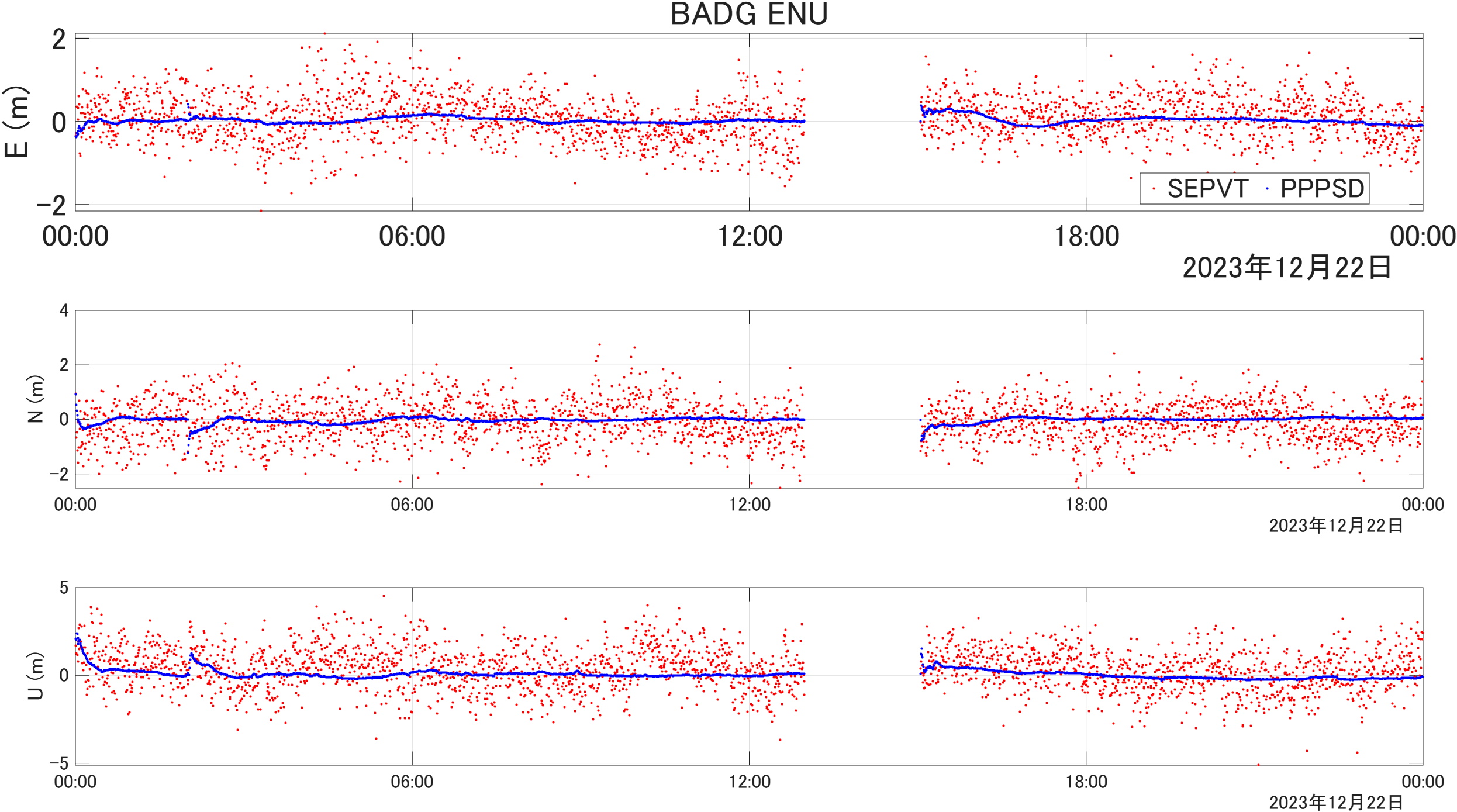
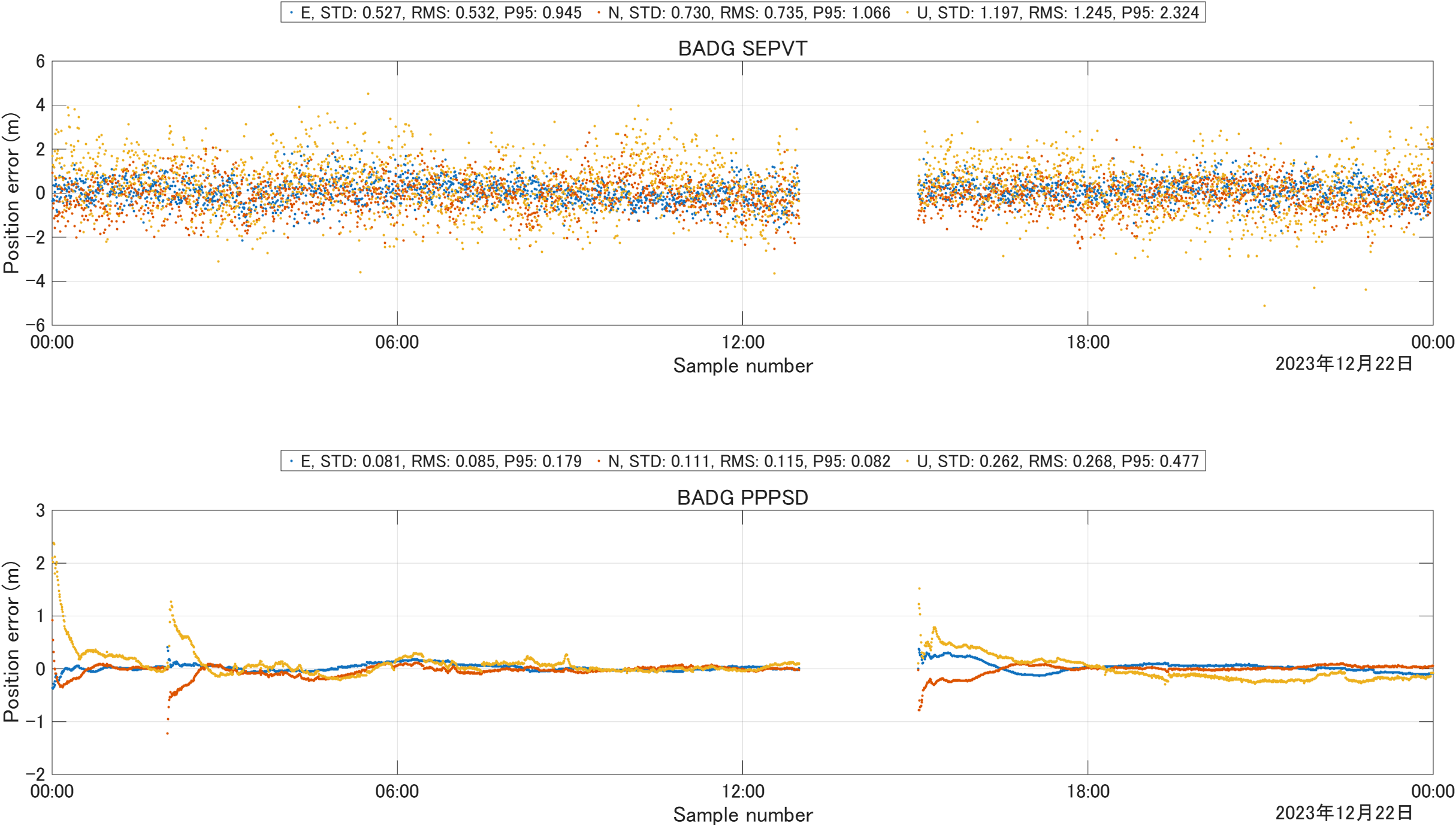
To plot the results, use Example_Plot_HASUA_PPPSD_stat_year_doy_any.m. When run, it asks for a station name and DOY and then shows the result directory. Clicking a MAT file in it displays 12 graphs one after another in about 30 seconds, as shown below. This example is for station BADG on December 22, 2023, with E6-B distribution (SIS).
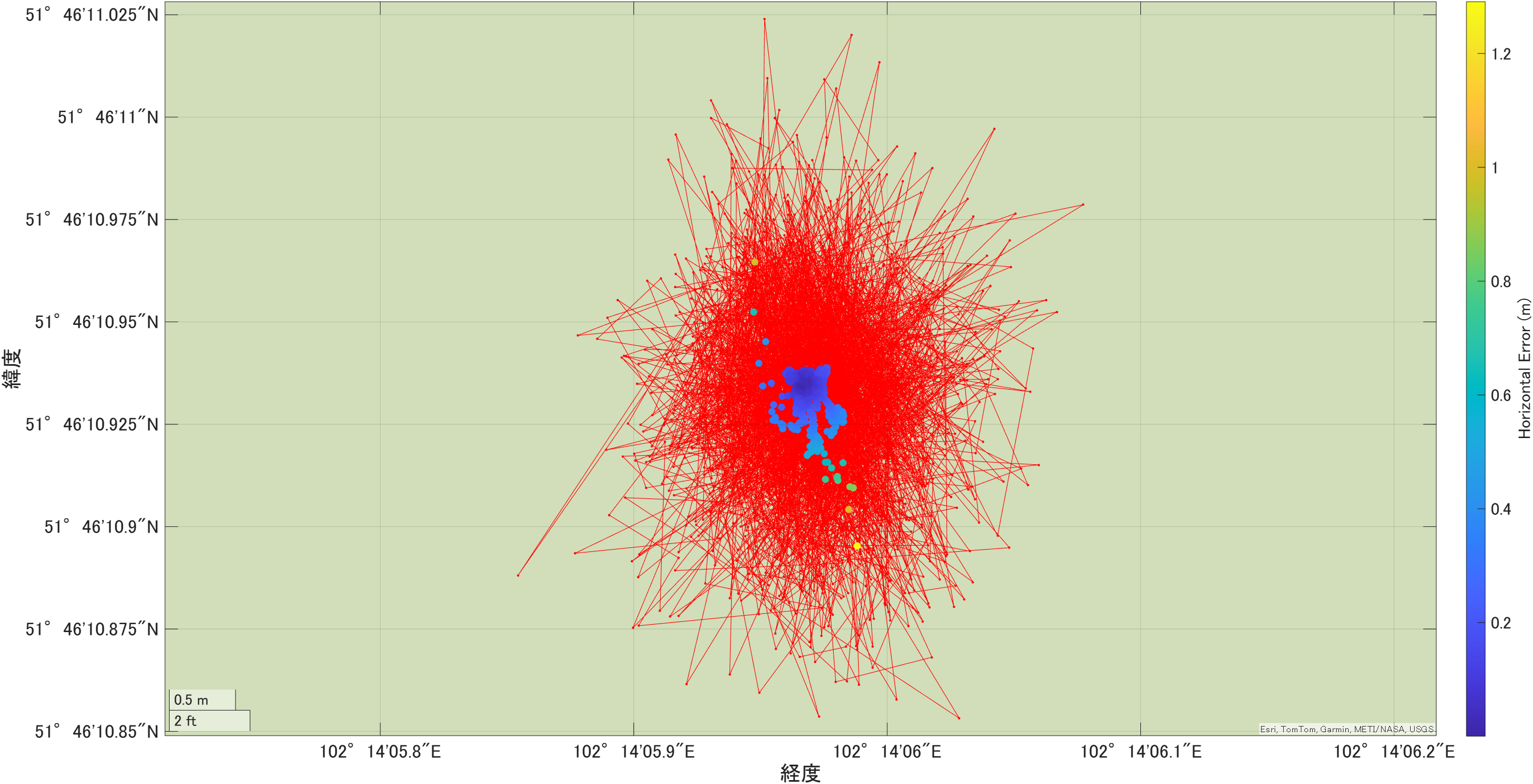
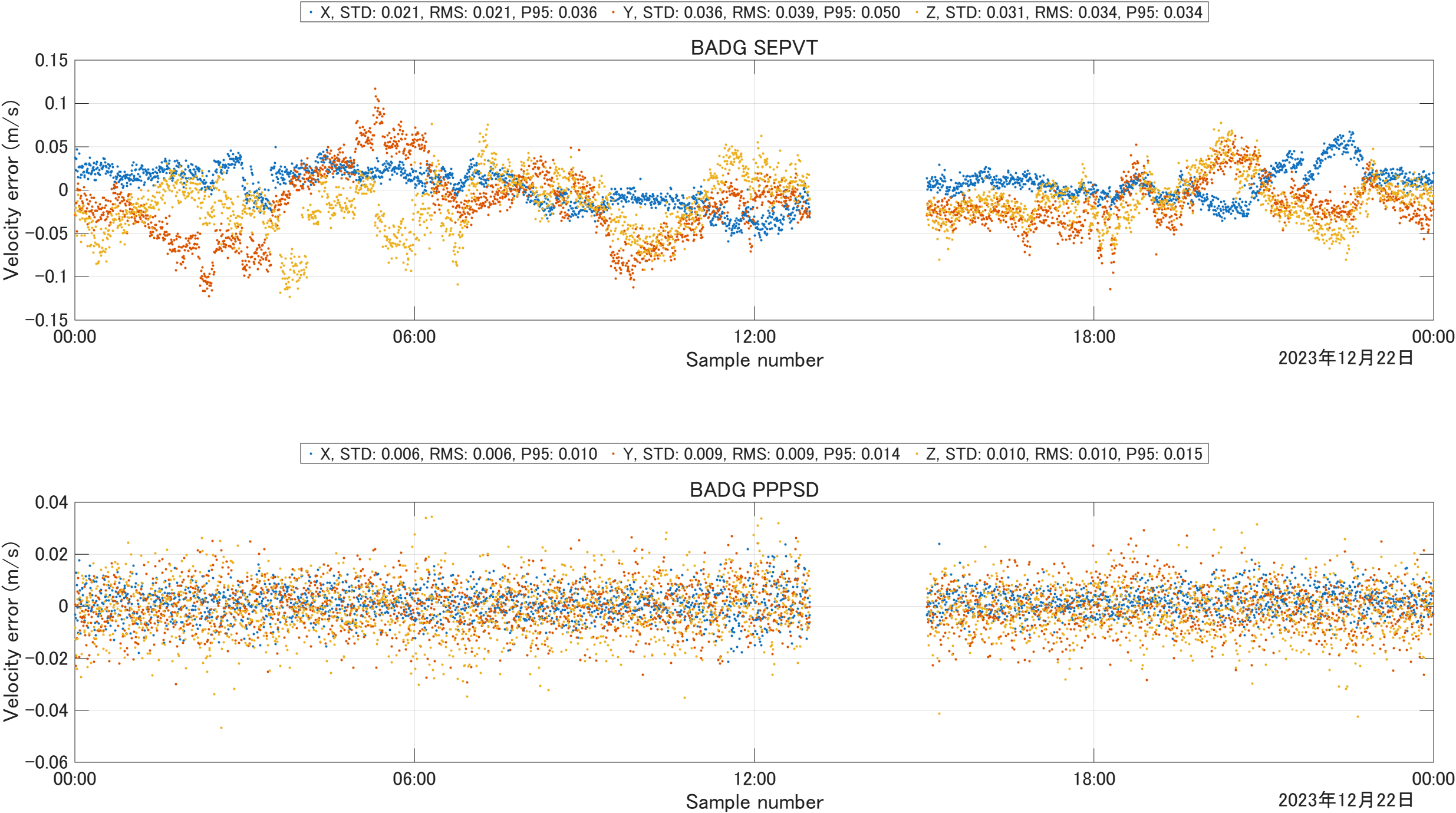
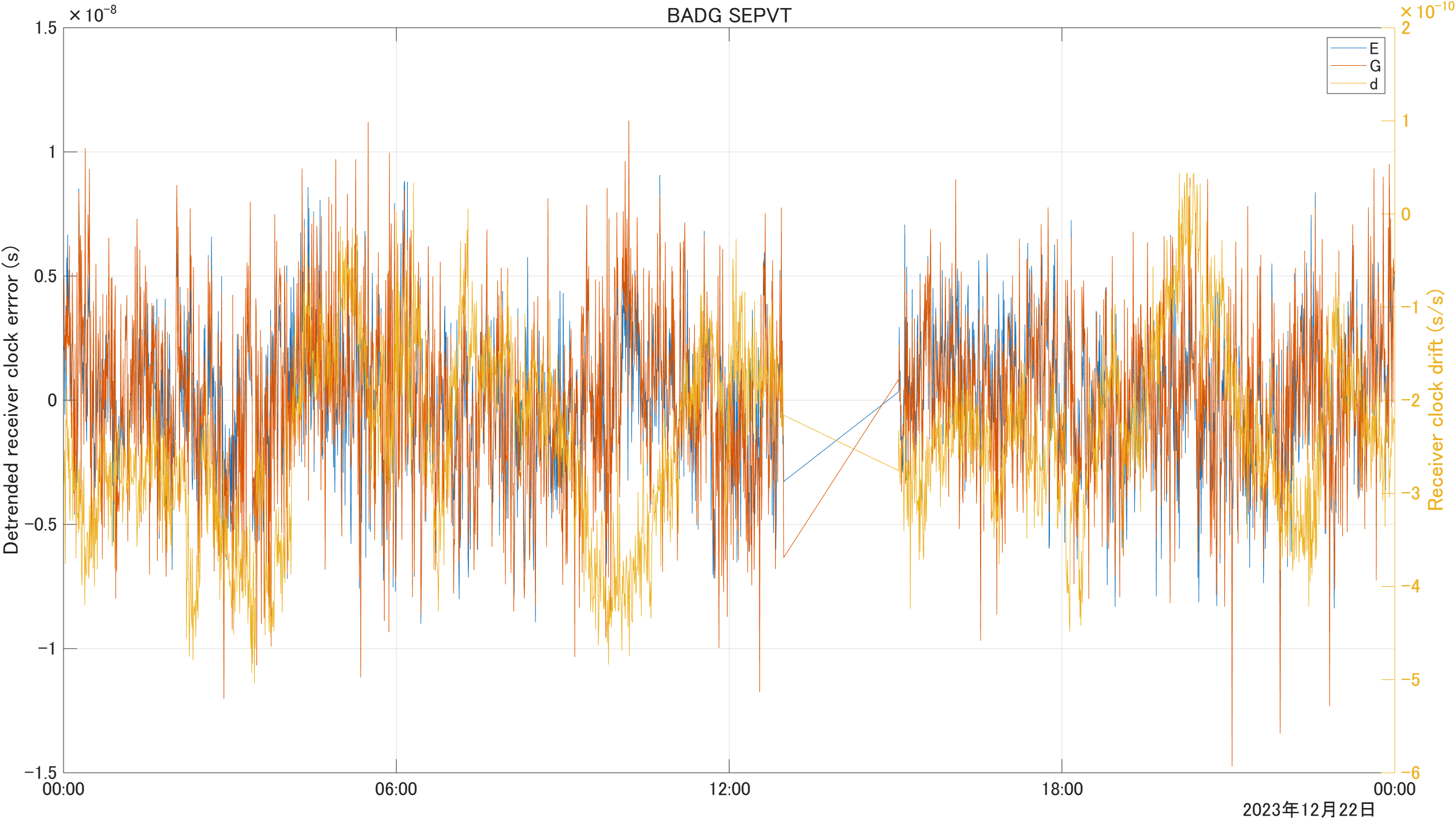
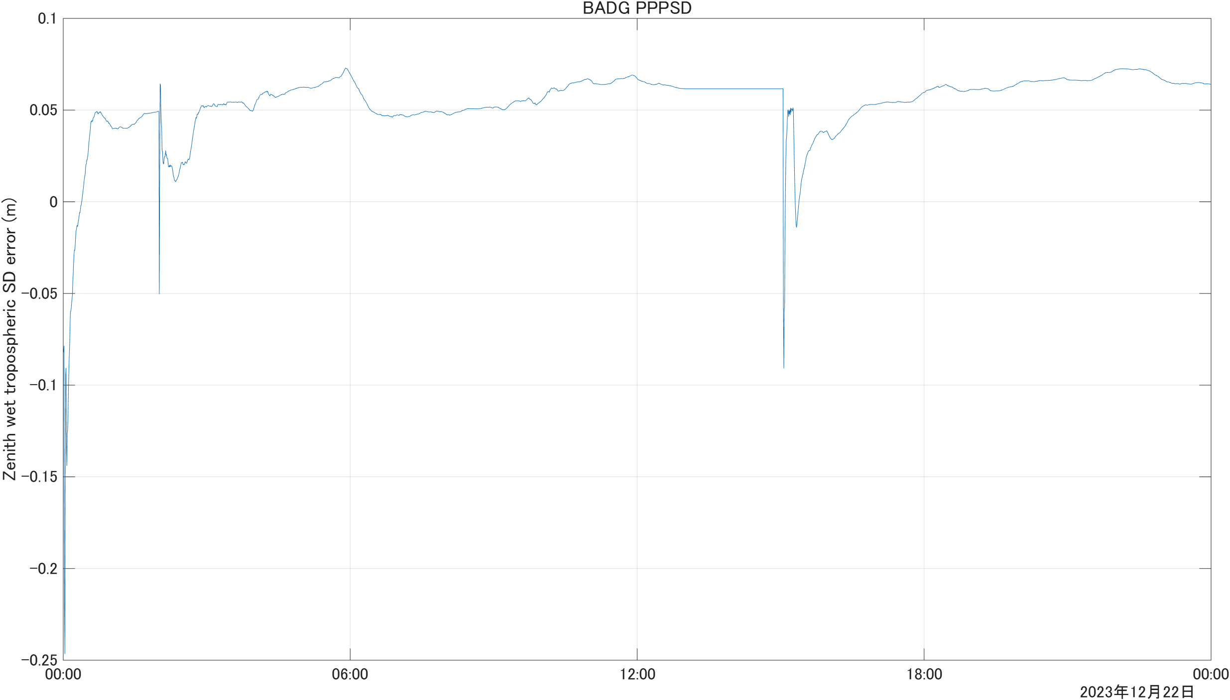
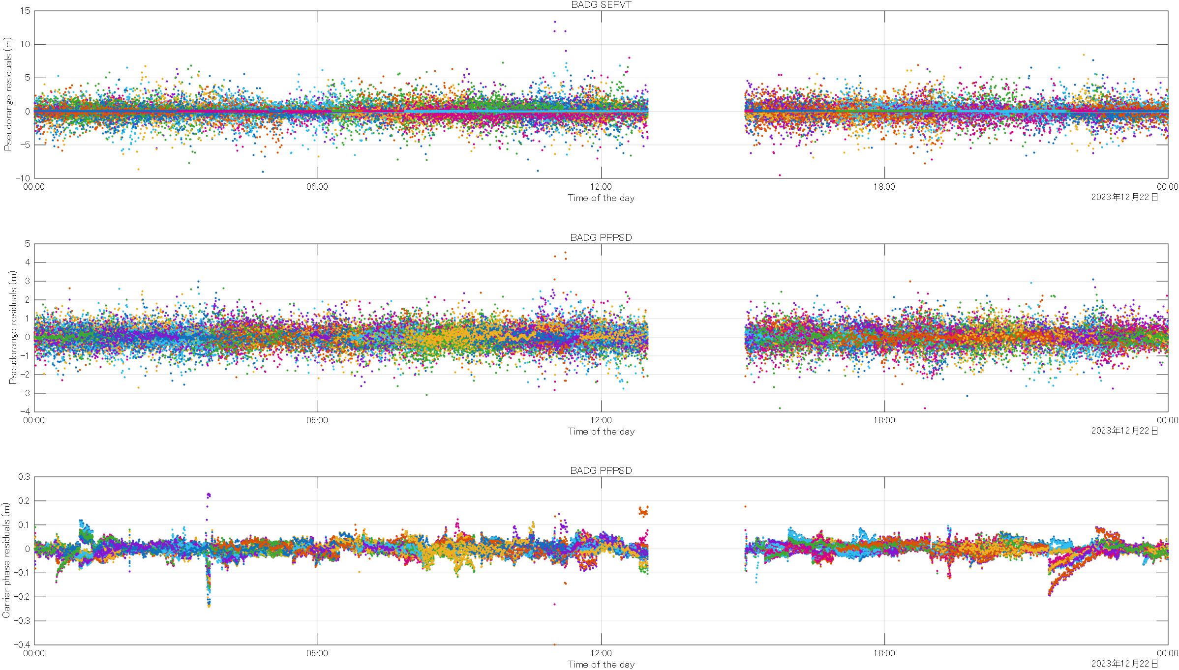
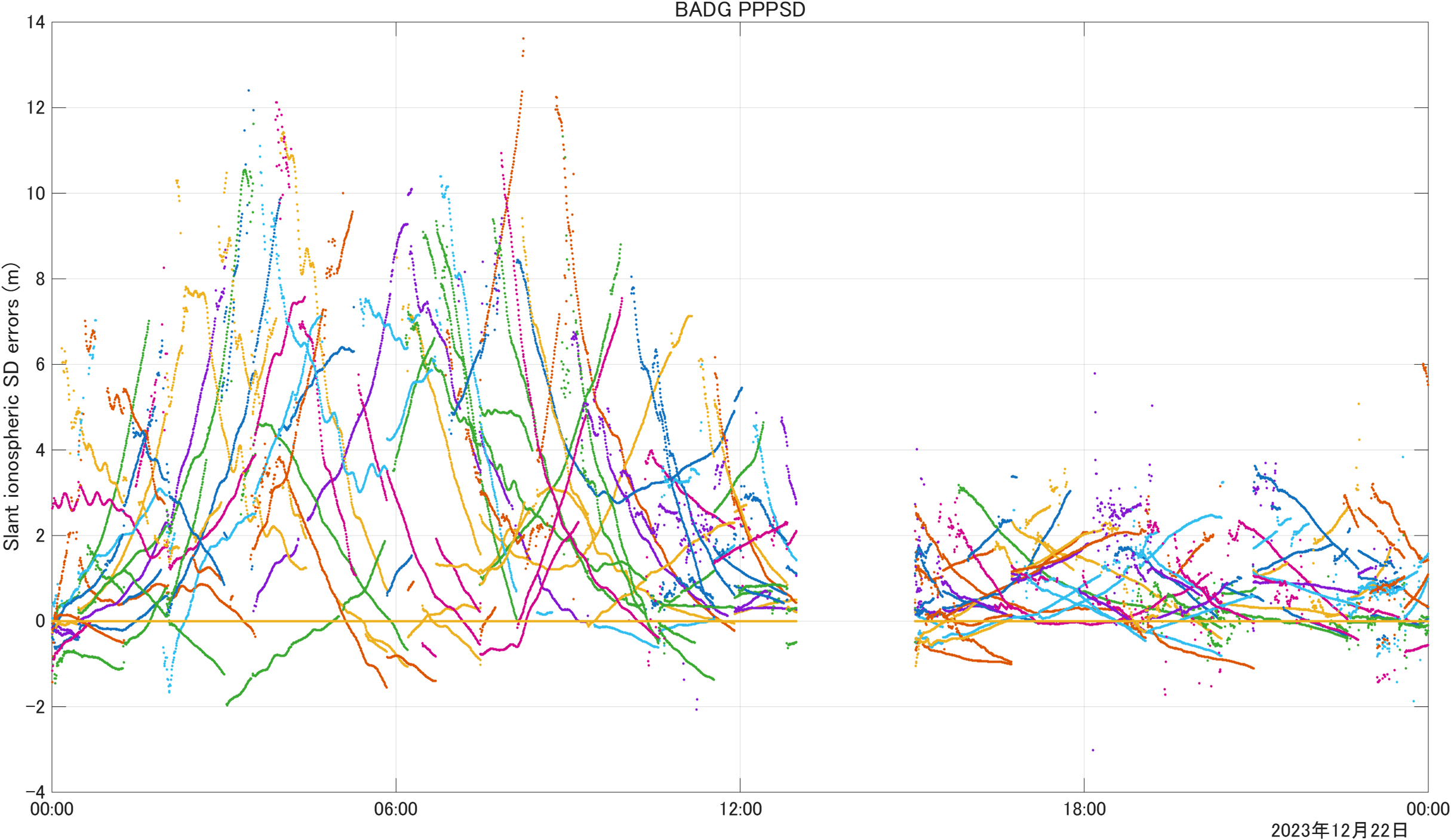
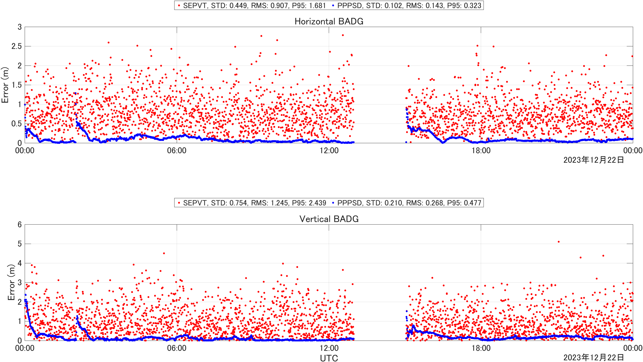
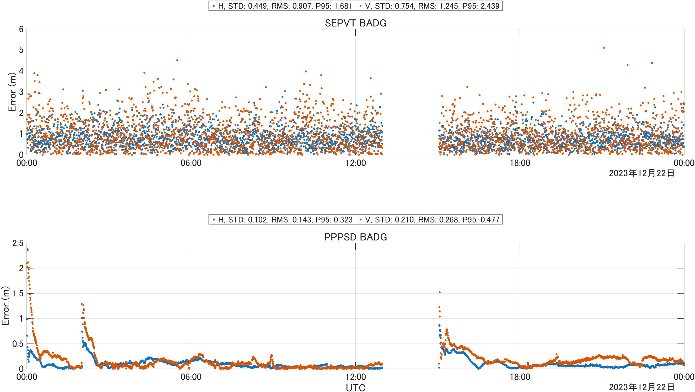
Many detailed analysis results were displayed. I would like to study them carefully and also try the software with my own data.
Conclusion
I tried the Galileo HAS performance evaluation software (HAS Reference User Algorithm). The software is written in MATLAB, and its source code can be read. The included data covered 6 stations over 10 days.
Related article(s):
- Galileo HAS(high accuracy service)Part 3 27th October 2023
- Galileo HAS(high accuracy service)part 2 20th February 2023
- Galileo HAS(high accuracy service)part 1 7th February 2023