Creating a positioning satellite skyplot using Python
Introduction
To know one’s coordinates using only radio waves from positioning satellites, positioning signals from at least four satellites are required. This is because four variables at the user’s position are unknown: latitude, longitude, ellipsoid height, and time.
It is preferable to be able to observe as many satellites as possible for positioning. I created a Python code that displays the positions of such positioning satellites in the sky.
Skyplot
For example, the satellite position display app [GNSS View] (https://qzss.go.jp/technical/gnssview/index.html) released by the Cabinet Office, Government of Japan, allows you to see the visible positions of positioning satellites at any location and any time. This is a screenshot of the position of the European Galileo satellites that will be observable in Hiroshima on November 23, 2023 at 23:20:00 UTC (November 24, 08:20:00 Japan time), plotted in GNSS View.
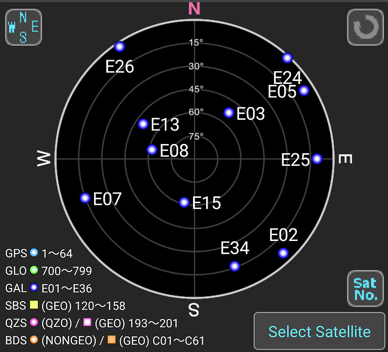
This diagram shows the direction and elevation angle at which positioning satellites can be seen from your own position, and is called a skyplot.
The open source GNSS-Radar, released by Professor Taro Suzuki of Chiba Institute of Technology, can display the positions of positioning satellites in a browser without an Internet connection. I use GNSS-Radar to find out the locations of positioning satellites.
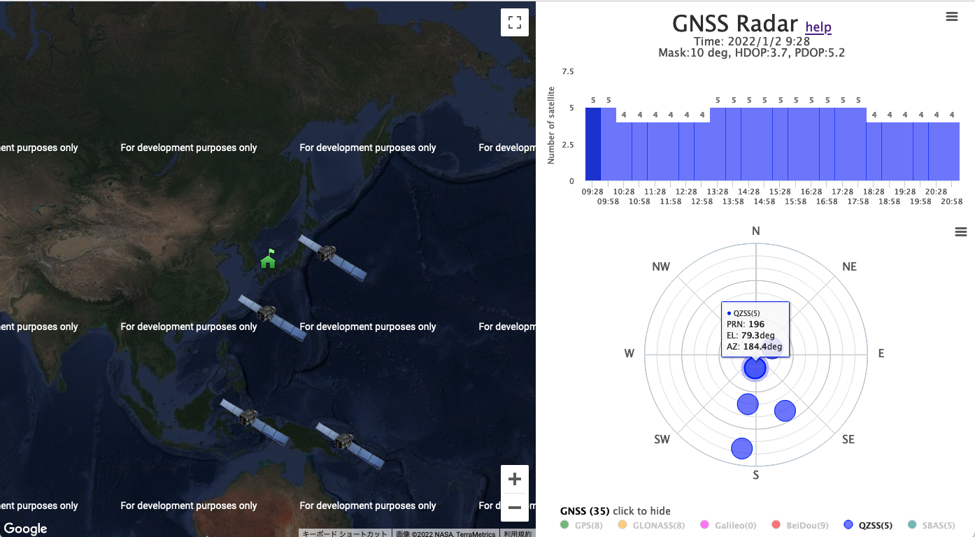
As you can see, there are several ways to know the locations of positioning satellites.
On the other hand, grayscale images in PDF format are preferable for creating reports, and you would like to create your own skyplots to highlight specific satellites and show observation conditions on the diagram. Also, to load such diagrams into, say LaTeX, a PDF file containing images in vector format is preferable, rather than a bitmap file such as a PNG or JPG file.
In order to create a skyplot with your own code, you will need to obtain the satellite orbits.
Two line element
Satellite positioning requires ephemeris, which shows the exact orbit of the satellite. On the other hand, to display a sky plot, it is sufficient to know the approximate satellite position, and for this purpose, two line elements (TLE) are often used. This is a two-line text format that shows the orbital inclination angle and other information required to represent the satellite orbit.
Such TLEs can be obtained from CelesTrak. Strictly speaking, satellite orbits may change from moment to moment, but unless orbital corrections are being made, the TLE is not expected to change significantly. The lifespan of an ephemeris is two hours, but once downloaded, the TLE can be used for a while. For example, the TLE of the recently launched Advanced Radar Satellite Daichi-4 is expressed as follows:
ALOS-4 (DAICHI-4)
1 60182U 24123A   24229.54940804  .00000500  00000+0  73855-4 0  9998
2 60182  97.9215 325.3457 0001395  98.1122  28.2230 14.79473854  6861
Here, we will try to obtain the TLEs of all European Galileo satellites from CelesTrak.
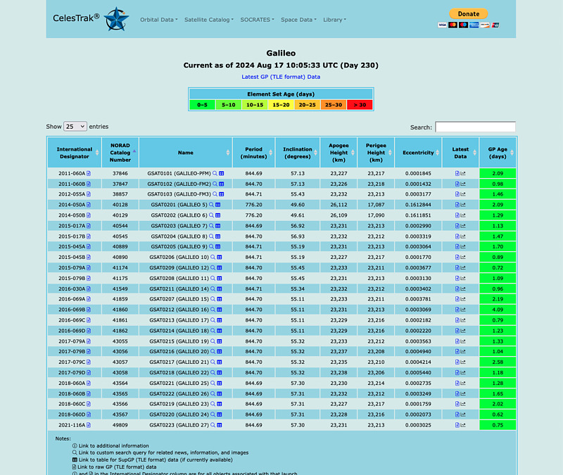
Click the document icon in the Latest Data column to display the TLE in your browser, then copy and paste it into a text file. Repeat this process for all Galileo satellites.
Skyplot creation using Python
Next, based on the TLE, we calculate the direction and elevation of the satellite from an arbitrary coordinate point. For coordinate calculation and display, we used Python’s non-standard modules skyfield, numpy, and matplotlib.
pip install skyfield numpy matplotlib
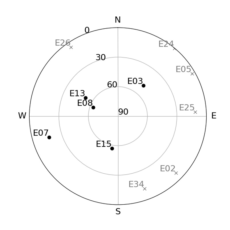
The code will display available satellites in the dictionary satellites1 with a circle, while unavailable satellites in satellites2 will be displayed with a cross. In addition, unavailable satellite numbers will be grayed out. In this example, the available satellites are E03, E07, E08, E13, and E15. E stands for Europe, which is a Galileo satellite. The order of the TLEs is arbitrary. The observation point is Hiroshima (coordinates 34.23N, 132.27E), and the date and time are 23:30:00 UTC on November 22, 2023.
skyplot.py
#! /usr/bin/env python
# -*- coding: utf-8 -*-

FILENAME = 'skyplot'
FONTSIZE = 16

# GAL TLE can be obtained from:
# https://celestrak.org/norad/elements/table.php?GROUP=galileo&FORMAT=tle

from skyfield.api import Topos, load, wgs84
from skyfield.sgp4lib import EarthSatellite
import numpy as np
from matplotlib import pyplot as plt
import datetime

# TLE data
satellites1 = {
"E03": ["1 41860U 16069B   24075.03714384  .00000000  00000+0  00000+0 0  9997",
    "2 41860  55.0417 123.9214 0003428 309.7138  50.3288  1.70474893 45607"],
"E07": ["1 41859U 16069A   24075.76931632 -.00000003  00000+0  00000+0 0  9996",
    "2 41859  55.0449 123.9045 0005163 290.7537  69.2607  1.70474715 45362"],
"E08": ["1 41175U 15079B   24077.45505889 -.00000001  00000+0  00000+0 0  9994",
    "2 41175  55.3797 123.8317 0004223 301.5343  58.4922  1.70474689 51340"],
"E13": ["1 43567U 18060D   24073.22747821 -.00000102  00000+0  00000+0 0  9991",
    "2 43567  57.3051   4.0560 0004572 309.8424  50.1177  1.70475162 35092"],
"E15": ["1 43564U 18060A   24073.15310948 -.00000102  00000+0  00000+0 0  9996",
    "2 43564  57.3028   4.0542 0005044 303.0742  56.8777  1.70475060 35093"],
}
satellites2 = {
"E11": ["1 37846U 11060A   24070.59038482 -.00000094  00000+0  00000+0 0  9990",
    "2 37846  57.1269   4.2009 0004048   0.9151 359.0813  1.70475681 76996"],
"E12": ["1 37847U 11060B   24075.36853573 -.00000108  00000+0  00000+0 0  9993",
    "2 37847  57.1277   4.0716 0005128 340.5417 117.7805  1.70475226 77083"],
"E19": ["1 38857U 12055A   24077.08212499 -.00000003  00000+0  00000+0 0  9991",
    "2 38857  55.3621 124.1355 0005270 267.6966  92.3107  1.70473587 70991"],
"E20": ["1 38858U 12055B   24075.29159274 -.00000001  00000+0  00000+0 0  9992",
    "2 38858  55.3626 124.1864 0002996 263.1608  96.8769  1.70473746 70965"],
"E18": ["1 40128U 14050A   24076.38068143 -.00000063  00000+0  00000+0 0  9995",
    "2 40128  49.7505 306.7902 1607231 147.6212 223.3476  1.85519539 63054"],
"E14": ["1 40129U 14050B   24077.17831918 -.00000057  00000+0  00000+0 0  9995",
    "2 40129  49.7668 305.8335 1605771 148.4561 222.2616  1.85520304 65236"],
"E26": ["1 40544U 15017A   24073.30254099 -.00000102  00000+0  00000+0 0  9991",
    "2 40544  56.9222   4.0745 0004144 291.6220  68.3342  1.70475448 55129"],
"E22": ["1 40545U 15017B   24074.14320105 -.00000105  00000+0  00000+0 0  9990",
    "2 40545  56.9283   4.0665 0003375 281.1733  78.7899  1.70475327 18189"],
"E24": ["1 40889U 15045A   24076.84456596  .00000028  00000+0  00000+0 0  9998",
    "2 40889  55.2656 244.3185 0005887  44.3383 315.6720  1.70473651 52993"],
"E30": ["1 40890U 15045B   24075.30543699  .00000030  00000+0  00000+0 0  9994",
    "2 40890  55.2642 244.3563 0003840  46.2777 313.7129  1.70473690 52990"],
"E09": ["1 41174U 15079A   24077.23534912 -.00000002  00000+0  00000+0 0  9999",
    "2 41174  55.3811 123.8397 0004688 303.6832  56.3397  1.70474783 50768"],
"E02": ["1 41549U 16030A   24076.99092123  .00000028  00000+0  00000+0 0  9995",
    "2 41549  55.4130 244.3111 0003383  18.6658 341.3102  1.70473716 48653"],
"E01": ["1 41550U 16030B   24076.10899448  .00000030  00000+0  00000+0 0  9998",
    "2 41550  55.4111 244.3364 0001211 357.6320   2.3289  1.70473751 48631"],
"E04": ["1 41861U 16069C   24077.75112543 -.00000001  00000+0  00000+0 0  9990",
    "2 41861  55.0457 123.8527 0005491 274.6415  85.3637  1.70473447 45518"],
"E05": ["1 41862U 16069D   24074.96434658  .00000001  00000+0  00000+0 0  9994",
    "2 41862  55.0430 123.9236 0004700 275.5406  84.4789  1.70474973 45591"],
"E21": ["1 43055U 17079A   24076.04030420  .00000030  00000+0  00000+0 0  9994",
    "2 43055  55.3883 244.1605 0000736  22.1381 337.8261  1.70474387 38952"],
"E25": ["1 43056U 17079B   24076.91865947  .00000028  00000+0  00000+0 0  9998",
    "2 43056  55.3883 244.1362 0001720 316.3645  43.5851  1.70474520 38986"],
"E27": ["1 43057U 17079C   24073.03300014  .00000027  00000+0  00000+0 0  9997",
    "2 43057  55.3924 244.2419 0002160 350.7256   9.2233  1.70474360 38903"],
"E31": ["1 43058U 17079D   24076.77253818  .00000029  00000+0  00000+0 0  9993",
    "2 43058  55.3864 244.1366 0001974 300.9948  58.9487  1.70474451 38996"],
"E33": ["1 43565U 18060B   24075.13123991 -.00000108  00000+0  00000+0 0  9993",
    "2 43565  57.3054   4.0028 0003358 282.1792  77.7846  1.70475082 35161"],
"E36": ["1 43566U 18060C   24073.59351374 -.00000103  00000+0  00000+0 0  9995",
    "2 43566  57.3052   4.0464 0004542 314.0609  45.9024  1.70475319 35115"],
"E34": ["1 49809U 21116A   24074.42529437 -.00000106  00000+0  00000+0 0  9990",
    "2 49809  57.2961   3.9185 0001376 281.4869 183.9787  1.70475239 14122"],
"E10": ["1 49810U 21116B   24075.39474642 -.00000108  00000+0  00000+0 0  9998",
    "2 49810  57.2968   3.8907 0001282 308.3744 144.5609  1.70475412 14162"],
}

# Load timescale and observer position
ts = load.timescale()
t = ts.utc(2023, 11, 22, 23, 30, 0)
observer = Topos(latitude_degrees=34.23, longitude_degrees=132.27)

# Initialize satellite objects
satellite_objects1 = {sat: EarthSatellite(satellites1[sat][0], satellites1[sat][1], sat, ts) for sat in satellites1}
satellite_objects2 = {sat: EarthSatellite(satellites2[sat][0], satellites2[sat][1], sat, ts) for sat in satellites2}

# Plotting
fig, ax = plt.subplots(subplot_kw={'projection': 'polar'},
    figsize=(6, 6))
ax.set_theta_zero_location('N')
ax.set_theta_direction(-1)
ax.set_ylim(0, 90)  # Altitude 0° (horizon) to 90° (zenith)

for sat in satellite_objects1:
    difference = satellite_objects1[sat] - observer
    topocentric = difference.at(t)
    alt, az, distance = topocentric.altaz()

    if alt.degrees > 0:  # Only plot if above the horizon
        r = 90 - alt.degrees
        theta = np.radians(az.degrees)
        ax.plot(theta, r, 'o', c='black')
        ax.text(theta, r, f'{sat}', fontsize=FONTSIZE, ha='right', va='bottom')

for sat in satellite_objects2:
    difference = satellite_objects2[sat] - observer
    topocentric = difference.at(t)
    alt, az, distance = topocentric.altaz()

    if alt.degrees > 0:  # Only plot if above the horizon
        r = 90 - alt.degrees
        theta = np.radians(az.degrees)
        ax.plot(theta, r, 'x', c='gray')
        ax.text(theta, r, f'{sat}', fontsize=FONTSIZE, ha='right', va='bottom', c='gray')

ax.set_rmax(90)
ax.set_rticks([0, 30, 60, 90])  # Altitude rings
ax.set_rlabel_position(-22.5)  # Move radial labels
ax.set_rgrids([0, 30, 60, 90], labels=["90", "60", "30", "0"], fontsize=FONTSIZE)
ax.grid(True)
ax.set_thetalim([0, 2*np.pi])
ax.set_thetagrids(np.rad2deg(np.linspace(0, 2*np.pi, 5)[1:]),
        labels=["E", "S", "W", "N"], fontsize=FONTSIZE)

plt.savefig(FILENAME + '.pdf')
#plt.savefig(FILENAME + '.svg')
#plt.savefig(FILENAME + '.tiff', dpi=600)
#plt.savefig(FILENAME + '.jpg', dpi=600)
#plt.savefig(FILENAME + '.png', transparent=True, dpi=600)

plt.show()
When you run this code with ./skyplot.py, the sky plot will be displayed on the screen and a PDF file of it will be output. By modifying the source code, you can change the output format to SVG, TIFF, JPG, or PNG, change the observation point or observation time continuously, or display various additional information.
Conclusion
I got the 2-line orbital elements TLE from CelesTrak and created a sky plot with my own Python code. With such a code at hand, you can create a sky plot of any satellite at any point, which is useful for various verifications.